
One of the issues with the boolean search model is that results are unranked - every matching document for a query contains all of the terms in that query, and there’s no real way of saying which are ‘better’. However, if we could weight the terms in a document based on how representative they were of the document as a whole, we could order our results by the ones that were the best match for the query. This is the idea that forms the basis for the vector space model.
Term Weights
The core problem is how we assign a weight to a term in a document. This could be as simple as keeping a count of appearances of the word in a document - so that a document that contains the term 10 times has a weight of 10, while one that contains it only twice has a weight of 2. This is referred to as the term frequency, and is a local weight - it can be calculated on a single document without referring to any others. This put a number to document for a given term by making the assumption that if a document refers to a term many times, then that term is probably indicative of it’s contents. However, it doesn’t take much practical examination to see that the term frequency will be high for words that we intuitively know are not indicative of contents: words like “the” or “a”.
The counterpart to this local weight, and countermeasure to the common-word problem, is the global weight, the weight of a term across many documents. One common global weight is inverse document frequency, which is defined as the count of all documents divided by the number of documents that contain the term. So, if there are 100 documents in the collection, and 9 of them contain the term in question, the idf of that term will be 11.1. This represents the observation that a term is more valuable in ranking a document if it is uncommon - a rare word is more likely to be indicative of a documents contents than a common one.
These weights are often combined into a tf-idf value, simply by multiplying them together. The best scoring words under tf-idf are uncommon ones which are repeated many times in the text, which lead early web search engines to be vulnerable to pages being stuffed with repeated terms to trick the search engines into ranking them highly for those keywords. For that reason, more complex weighting schemes are generally used, but tf-idf is still a good first step, especially for systems where no one is trying to game the system.
There are a lot of variations on the basic tf-idf idea, but a straightforward implementation might look like:
<?php
$tfidf = $term_frequency *  // tf
        log( $total_document_count / $documents_with_term, 2); // idf
?>
It’s worth repeating that the IDF is the total document count over the count of the ones containing the term. So, if there were 50 documents in the collection, and two of them contained the term in question, the IDF would be 50/2 = 25. To be accurate, we should include the query in the IDF calculation, so if in the collection there are 50 documents, and 2 contain a term from the query, the actual calculation would be 50+1/2+1 = 51/3, as the query becomes part of the collection when we’re searching.
We take logs of the IDF to provide some smoothing. If a term A is represented in x document, and term B 2x times, then term A is a more specific term that should provide better results, but not necessarily twice as a good. The log smooths out these differences.
Document Similarity
Once we have a weight calculated (or calculatable) for all the terms, we actually have a kind of matrix, or table, for our document collection, most entries of which are zero, because any given document will only contain a small percentage of all the words we’ve encountered in a large collection - the matrix can be described as sparse. Because of this excess space, and for other reasons covered in boolean search, we’ll store it as a term => document mapping:
<?php
function getIndex() {
        $collection = array(
                1 => 'this string is a short string but a good string',
                2 => 'this one isn\'t quite like the rest but is here',
                3 => 'this is a different short string that\' not as short'
        );

        $dictionary = array();
        $docCount = array();

        foreach($collection as $docID => $doc) {
                $terms = explode(' ', $doc);
                $docCount[$docID] = count($terms);

                foreach($terms as $term) {
                        if(!isset($dictionary[$term])) {
                                $dictionary[$term] = array('df' => 0, 'postings' => array());
                        }
                        if(!isset($dictionary[$term]['postings'][$docID])) {
                                $dictionary[$term]['df']++;
                                $dictionary[$term]['postings'][$docID] = array('tf' => 0);
                        }

                        $dictionary[$term]['postings'][$docID]['tf']++;
                }
        }

        return array('docCount' => $docCount, 'dictionary' => $dictionary);
}
?>
Knowing this represents each document as a list of numbers though allows us to view the documents as something slightly different. We can treat each document as if it is a point on a graph, with a number of axes equal to the number of different terms we know about. We can treat it as a point in a space with a very high number of dimensions, but if we just take the first two terms, we can plot the documents against each other on a standard XY graph to compare the relative position of the two documents:
We can use the dictionary we built above to determine the positions - the weights - of the documents in the X (‘short’) and Y (‘string’) dimensions.
<?php
function getTfidf($term) {
        $index = getIndex();
        $docCount = count($index['docCount']);
        $entry = $index['dictionary'][$term];
        foreach($entry['postings'] as  $docID => $postings) {
                echo "Document $docID and term $term give TFIDF: " .
                        ($postings['tf'] * log($docCount / $entry['df'], 2));
                echo "\n";
        }
}
?>
This gives us:
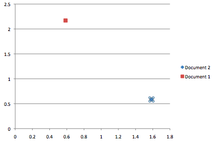
Document 1 and term short give TFIDF: 0.584962500721
Document 3 and term short give TFIDF: 1.58496250072
Document 1 and term string give TFIDF: 2.16992500144
Document 3 and term string give TFIDF: 0.584962500721
We can compare these two documents by plotting them. Note that one document is not listed, but would be at 0,0 as it doesn’t contain either term.
Once we extend this concept to include of the terms we collected as we were indexing, every document becomes a point in a space with an awful lot of dimensions.We can even treat our query as a point in this very high dimension space, and then compare documents to it by calculating how far away they are.
We might look for the 10 closest documents, and return then as our search results. However, just comparing the distance can cause problems when documents are different lengths. Doubling a document, adding itself to itself, shouldn’t really effect how similar it is to another document, but it’s likely to move it quite a way away.
So, instead of considering our documents as points in this space, we think about them as vectors, lines going from the origin (the 0 point in the space, like {0,0,0} in the three dimensional space) to the point defined by their weights. The similarity can then be determined by how close the two lines are to each other.
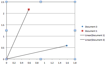
We also normalise by dividing each component by the length of the vector, so that they all have a length of 1, unit length.
<?php
function normalise($doc) {
        foreach($doc as $entry) {
                $total += $entry*$entry;
        }
        $total = sqrt($total);
        foreach($doc as &$entry) {
                $entry = $entry/$total;
        }
        return $doc;
}
?>
The advantage of this bit of maths is that we can then use another measure to calculate the similarity between two documents, or, more relevantly, a document and a query, the cosine similarity. By taking the dot product between the two vectors we get the cosine of the angle between the two lines. This will be -1 for vectors pointing in opposite directions, 0 if they’re at 90 degrees to each other, and 1 if they are identical - i.e. there is no angle between them. This conveniently means the documents with the highest values relative to a query are the best matches - their vectors are pointing in the same direction as the query vector.
Calculating the dot product is actually really simple, just a case of multiplying each component in the vector with it’s counterpart in the other vector, and adding all the results. So, for example, {.0.5,0.4,0.1} dot {0.5, 0.1, 0.4} = 0.5*0.5 + 0.4*0.1 + 0.1*0.4 = 0.25 + 0.04 + 0.04 = 0.33
<?php
function cosineSim($docA, $docB) {
        $result = 0;
        foreach($docA as $key => $weight) {
                $result += $weight * $docB[$key];
        }
        return $result;
}
?>
This is a nice robust similarity score, and this way of viewing the document collection is what is referred to as the vector space model. There are plenty of improvements to be made, such as better weighting schemes, and a lot of implementation difficulties to consider, but the model provides a way of getting good results from natural queries, which don’t have boolean operators.
Of course, we don’t want to compare every document to the query, so we return to our positing lists to retrieve all the documents that share any of the terms with the query (any dimensions not shared would give a dot product of 0 anyway). Once we have that, we can take advantage of the fact that we’re not looking for an exact cosine similarity, just one relative to other documents. This means we can accumulate document matches to get a final ranked score, which saves us some comparison effort, effectively setting the weight of each term in the query to 1.
The code below performs this kind of search, for the query “is short string”.
<?php
$query = array('is', 'short', 'string');

$index = getIndex();
$matchDocs = array();
$docCount = count($index['docCount']);

foreach($query as $qterm) {
        $entry = $index['dictionary'][$qterm];
        foreach($entry['postings'] as $docID => $posting) {
                $matchDocs[$docID] +=
                                $posting['tf'] *
                                log($docCount + 1 / $entry['df'] + 1, 2);
        }
}

// length normalise
foreach($matchDocs as $docID => $score) {
        $matchDocs[$docID] = $score/$index['docCount'][$docID];
}

arsort($matchDocs); // high to low

var_dump($matchDocs);
?>
The result is as we expect:
array(3) {
  [1]=>
  float(0.804028972103)
  [3]=>
  float(0.74553272203)
  [2]=>
  float(0.211547721742)
}
This is a quick and easy way of generating search results, and isn’t a million miles away from the way the something like MySQL’s full text indexing, or a lot of other search engines, work.