
Monte Carlo simulations are a handy tool for looking at situations that have some aspect of uncertainty, by modelling them with a pseudo-random element and conducting a large number of trials. There isn’t a hard and fast Monte Carlo algorithm, but the process generally goes: start with a situation you wish to model, write a program to describe it that includes a random input, run that program many times, and look at the results.
In each case, you’re taking a pot shot at the result, and over many iterations you should get a broad picture of the probabilities of certain outcomes. If these match observations of the real situation, your model is a good one. Alternatively, if you can achieve certain results through randomness that others put down to some other factor, perhaps there is more chance in the real situation that others have expected.
As an example, lets imagine visiting an SEO expo, filled with 10,000 SEO experts. Now, 20% of the experts are creative copywriters and link profile experts who will help to make your site more usable, more readable, faster, and help drive traffic from disparate sources as they improve your search profile. The others are clueless keyword stuffers and link spammers, who will turn your site into an real mess.
However, a given rank on a results page is dependent on an awful lot of things - how the site was originally, what other sites are doing, changes to google’s algorithms, temporary network and server effects and so on. Because of that, sometimes the bad SEOs get their sites onto the front page, and sometimes the good ones don’t. Let estimate that the good SEOs get their site onto the first page under a given term two thirds of the time, while for the bad SEOs it’s only one third of the time. Now, whichever SEO you ask claims to be in the good category, of course, so you ask to see the results for the last 5 sites they optimised. If they are all on the first page, can you be confident you’ve got a good one?
We can set up a monte carlo simulation for that by simply looping over the five sites, and seeing which ones succeed each time, by chance, and which fail. Starting with our total 10,000 SEO population, how many good vs bad SEOs do we expect.
<?php
$tGood = $tBad = 0;
$iterations = 10000;

for($iters = 0; $iters < $iterations; $iters++) {
        $goodCount = 2000;
        $badCount = 8000;

        for($i = 0; $i < 5; $i++) {
                $max = $goodCount;
                for($j = 0; $j < $max; $j++) {
                        if(lcg_value() < 0.33) {
                                $goodCount--;
                        }
                }
                $max = $badCount;
                for($j = 0; $j < $max; $j++) {
                        if(lcg_value() < 0.66) {
                                $badCount--;
                        }
                }
        }
        $tGood += $goodCount;
        $tBad += $badCount;
}

var_dump("Good SEOs: " . $tGood/$iterations);
var_dump("Bad SEOs: " . $tBad/$iterations);
?>
After our 10,000 iterations, we see the numbers come out with a majority of good SEOs, but some bad ones have made it through:
string(19) "Good SEOs: 270.0382"
string(16) "Bad SEOs: 36.343"
This is an example where we can use brute force to solve what would otherwise be an integration problem. Admittedly, this is not a very difficult problem, but the logic can be continued and refined into situations that are require more complex maths. The wikipedia Monte Carlo simulator page has a good description of how the value of Pi can be estimated by a Monte Carlo method, for example.
Projecting The Future
For a more complicated example, we can think about planning a development project. We’d like to take a set of estimates, and run them through a Monte Carlo simulation to see what kind of overall times we can expect. Imagine that we’ve taken a look at past projects, and concluded a few things about the estimate. Our estimates always come in a ‘best case’, ‘worst case’ variety, so we have a range of numbers. Most tasks are delivered somewhere within that range, usually well under the worst case, but there are small few that seem to go way over it.
We decide to model this by assuming that worst case is actually 3 times that estimated originally. However, rather than assuming we have equal chance of getting any value in that range (a flat distribution), we want to model our chance of getting the lower results as being higher than getting the higher ones. This kind of distribution is called a power law, and we can use a function that models that distribution for our random function.
<?php
function powerLaw($min, $max, $n) {
        $max += 1;
        $val = pow(
                        ( pow($max, $n+1) - pow($min, $n+1) )
                                * lcg_value()
                                + pow($min, $n+1),
                        (1.0/($n+1))
                );
        return $max - 1 - $val + $min;
}

function getTotalTime($estimates) {
        $totalTime = 0;
        foreach($estimates as $estimate) {
                $totalTime += powerLaw($estimate['best'], $estimate['worst']*3, 5);
        }
        return $totalTime;
}
?>
With those functions in place, all we have to do is feed in our estimates, and for each one run them through the getTotalTime function. We can do a number of loops of this, and look at the results that we get.
<?php
// our estimates
$estimates = array(
        "login form" => array("best" => 2, "worst" => 10),
        "forgotten password" => array("best" => 8, "worst" => 20),
        "profile page" => array("best" => 16, "worst" => 20),
        "avatar upload" => array("best" => 8, "worst" => 14),
);

// conduct 10,000 trials
$results = array();
for($i = 0; $i < 10000; $i++) {
        $res = getTotalTime($estimates);
        if(!isset($results[$res])) {
                $results[$res] = 0;
        }
        $results[$res]++;
}
ksort($results);
?>
This gives us an array of results, from which we can calculate some estimates. For example, although the worst case from the estimates is 64 hours, if we want to account for 80% of the runs we’d need to allocate around 68 hours - and assuming our model is correct then our project would still have a 20% chance of going over!
We can visualise this by using the Google Charts API, which helps to show how, while the bulk of runs fit around the original hours, there is a tail to consider of unexpectedly long delivery times:
<?php
$url = “http://chart.apis.google.com/chart?chs=450x200&cht=bvs”;
$url .= ‘&chds=0,’ . max($results);
$url .= ‘&chd=t:’ . implode(“,”, $results);
$url .= “&chbh=3,1,1”;
echo $url; // url for google
?>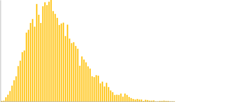
The length of time runs along the horizontal access, number of trials that resulted in that time in the vertical access. The long tail of growing times of the estimate show why to get a more certain timescale we have to go way over our original worst case, but still having the project likely to be delivered somewhere in the original range.
The nice thing about these methods is that they are fairly easy to get a grip of. You can plug in a randomness function of your choosing based on almost anything, and try modelling situations that otherwise would be hard to understand intuitively. By plotting the result of calculating statistics you can quickly try out scenarios and get a feel for different sort of effects, as long as there’s an element in the thing you are modelling that is chaotic enough to be effective random.